Source Time Series

The time series for a source is edited on this form. A source can have an overall time series representing a single event, such as the firing of an airgun.

Data Import

Data may be imported from a WAV file. The WAV file’s sampling rate will be used. For stereo files, the first (left) channel is imported. WAV samples are normalised to the range -1.0 to 1.0 on import, so the pressure must be scaled afterwards: enter the peak pressure in pascals corresponding to full scale in the Scale pressure by: field and click the button. The factor is a plain multiplier and can also be applied to text data.

Alternatively, data can be imported from a text file containing the individual samples on separate lines. The values should be given in Pascals, as shown in the example below. A text file carries no sample rate, so enter it in the Sample rate (Hz) field before importing (if left blank, 44 100 Hz is assumed).

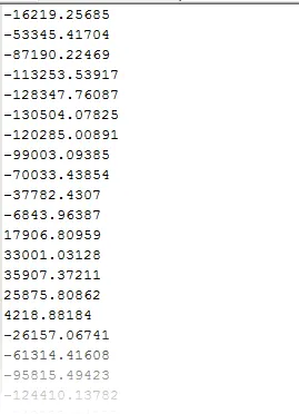Image 1: Example of time series samples in Pascals.

The sample rate is used to filter the signal into frequency bands; bands that cannot be resolved at the given sample rate are shown as a dash (see the FAQ on sample rates). The Count value specifies the number of impulse events (e.g. pile strikes) and adds 10·log₁₀(Count) to the SEL. For a moving source it applies at each calculation position, so the total number of events is positions × Count.

After import, the form displays the derived levels: single-event SEL (dB re 1 µPa²·s at 1 m, with the Count contribution shown separately), SPL peak and SPL peak-to-peak (dB re 1 µPa at 1 m), along with the frequency band breakdown.

Mitigation

Mitigation is entered for each frequency band, and dBSea recalculates the band-filtered time series data with these mitigation values during the solve phase. As with the source spectrum page, positive values of mitigation result in a reduction of sound level in that frequency band.

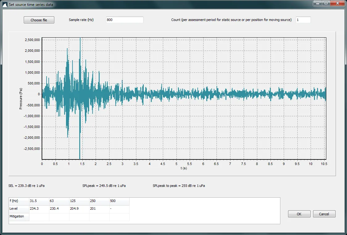Image 2: Source time series form used for mitigation adjustments.