Solvers

dBSea offers a range of calculation methods (solvers). The 3D solvers are recommended for most work. 2D solvers are available for legacy projects or simpler scenarios.

For detailed technical background on these methods, see Computational Ocean Acoustics. Jensen et al., Springer, 2011.

Solver Overview

Solver	Best For	Time Domain	Directivity Support
dBSeaPE 3D	Low frequency, complex environments	Yes (broadband PE)	Yes
dBSeaRay 3D	High frequency, complex environments	Yes (ray arrivals)	Yes
dBSeaPE (2D)	Legacy projects	Yes (broadband PE)	Yes
dBSeaRay (2D)	Legacy projects	Yes (ray arrivals)	Yes
20 log / 10 log	Quick estimates	No	No

Split Low/High Frequency Solvers

Different solvers may be chosen for low and high frequency ranges. The crossover frequency is set on the Frequencies and Solvers page. The only recommended split configuration is PE for low frequencies and Ray for high frequencies — the reverse (Ray low, PE high) should never be used, as Ray cannot accurately model low-frequency propagation in shallow water and PE becomes impractically slow at high frequencies.

In general, keep the crossover frequency as low as practical. PE solve time increases quadratically with frequency, so pushing the PE solver to higher bands significantly increases computational load. However, the Ray solver has a depth-dependent low-frequency cutoff — in shallow water you may need PE to handle a wider frequency range.

The crossover frequency can be estimated as:

$f = \frac{8d}{c}$

where f is the frequency in Hz, d is the average depth in meters, and c is the speed of sound (m/s). Experimentation may be required where depth varies significantly.

Seawater Attenuation

The solver-calculated transmission loss includes attenuation with distance in seawater. This is negligible at low frequencies but becomes significant at high frequencies—approximately 30 dB/km at 100 kHz. The attenuation curve is shown on the Water page.

3D Parabolic Equation Solver (dBSeaPE 3D)

The 3D parabolic equation solver is recommended for low-frequency problems. It provides full 3D propagation modeling, properly handling environments where bathymetry or properties vary in all directions.

Key characteristics:

Collins’ split-step solver for accurate wide-angle propagation
Collins’ self-starter for reliable initialization across frequency ranges
Improved Padé series coefficient calculation for numerical stability
Range-dependent bathymetry and environmental properties
The sediment layer extends to twice the water column depth, with attenuation increasing at depth to absorb energy at model boundaries
The sea surface is modeled as a pressure-release interface
Source directivity support

3D Ray Tracing Solver (dBSeaRay 3D)

The 3D ray solver is recommended for high-frequency problems. It traces rays from the source through the full 3D environment.

Key characteristics:

Traces individual ray paths through the 3D environment, accounting for refraction from sound speed gradients and reflection from the surface and seafloor
Accurate ray phase calculation at each update point — phase shifts along each path are tracked, enabling coherent summation of ray contributions
Ray arrival lists — per-frequency arrival information at receiver points, providing propagation time delays for each path
Coherent or incoherent summation of ray contributions (configurable)
Robust ray termination conditions
Optimized default settings for common use cases
Source directivity support

Configuration

The number of rays and summation method (coherent or incoherent) can be set in Preferences → Solver advanced
Setting the ray count to 0 lets the solver choose automatically
Using a low ray count for initial tests, then increasing for the final solve, is often practical

Seafloor Reflections

For multiple seafloor layers, rays are not traced into the seabed. Instead, a complex reflection coefficient representing the layer stack is applied at each seafloor reflection, following Jensen et al. (2011), section 1.6.

Time-Domain Calculations (Ray)

The ray solver supports time-domain calculations. Rather than returning transmission loss at each point, the solver returns ray arrival lists (per frequency). These can be used to calculate time series at receiver points, from which peak, peak-to-peak, and frequency band SEL levels are derived.

Species Weighting in Time-Domain Solves

How species weighting is applied depends on the metric type, following NOAA/NMFS guidance:

SEL (time): The selected species weighting is applied per frequency band before summing across bands. This is consistent with the filterbank approach used in the NOAA framework and matches the weighting behaviour in frequency-domain solves.
SPL peak / peak-to-peak: No weighting is applied. Under NOAA/NMFS guidance, peak SPL is an unweighted (flat) metric — the peak pressure of the broadband waveform is reported directly regardless of any species weighting selection.

For frequency-domain solves, the selected species weighting (or none) is always applied as usual.

Time-Domain Calculations

Both the PE and Ray solvers support time-domain calculations. A scenario can use a single solver or a split solver configuration for time-domain work:

Single solver: Either PE (for low frequencies) or Ray (for high frequencies) can be used alone for time-domain solves.
Split solver: PE handles the low-frequency bands and Ray handles the high-frequency bands. Only this direction is valid — never assign Ray to low frequencies or PE to high frequencies in a split configuration.

In a split solver time-domain solve, a single source time series is used for both solvers. dBSea automatically extracts the relevant spectral content for each solver’s frequency range — there is no need to prepare separate source data for the low and high bands.

How Time-Domain PE Works

The PE solver computes time-domain results using broadband synthesis. The PE is solved at many closely-spaced frequencies (oversampled relative to the output bands), the complex transfer function is multiplied by the source spectrum, interpolated to a linear frequency grid, and an inverse FFT produces a pressure time series at each receiver point.

The frequency oversampling rate is configurable under Advanced PE Solver Options: 1/3, 1/6, 1/12, or 1/24 octave spacing. Compute time scales with the denominator (1/24 takes roughly 4× longer than 1/6). The default of 1/6 octave works well in most cases — the acoustic transfer function envelope varies slowly enough across frequency that finer spacing rarely changes the result.

Time-Domain Metric Types

Before starting a time-domain solve, you must choose the output metric. The metric type cannot be changed after solving — a fresh solve is required to switch between them.

Metric	Description	Per-band spectrum available?
SEL (time)	Sound exposure level integrated over the time series	Yes
SPL peak (Lp)	Peak instantaneous pressure level	No
SPL peak-to-peak (Lp-p)	Difference between maximum and minimum pressure	No

Species Weighting in Time-Domain Solves

How species weighting is applied depends on the metric type, following NOAA/NMFS guidance:

SEL (time): The selected species weighting is applied per frequency band before summing across bands. This is consistent with the filterbank approach used in the NOAA framework and matches the weighting behaviour in frequency-domain solves.
SPL peak / peak-to-peak: No weighting is applied. Under NOAA/NMFS guidance, peak SPL is an unweighted (flat) metric — the peak pressure of the broadband waveform is reported directly regardless of any species weighting selection.

For frequency-domain solves, the selected species weighting (or none) is always applied as usual.

2D Solvers (Legacy)

The 2D solvers (dBSeaPE and dBSeaRay) use radial symmetry, calculating propagation in slices radiating from each source. They are retained for compatibility with older projects.

For new work, use the 3D solvers instead.

Simple Geometric Spreading

For quick estimates, simple geometric spreading models are available:

20 log - Spherical spreading (inverse square law). Frequency-independent, ignores bathymetry.
10 log - Cylindrical spreading beyond the water depth at the source. Frequency-independent.

These are useful for initial estimates but do not account for environmental effects.

Deprecated Solver

dBSeaModes

Note: The normal modes solver is deprecated. For low-frequency modeling, use the PE solvers instead.

Existing projects using dBSeaModes will still open, but consider switching to dBSeaPE 3D for new work.

Postprocessing

After solving, transmission losses for each source are post-processed. These steps are optional and can be controlled in Preferences → Solver advanced:

Monotonic decrease - Transmission loss is constrained to decrease monotonically with distance from the source
Radial smoothing - Transmission loss is averaged radially using a triangular kernel

To disable, set the radial smoothing factor to 0 and uncheck “Levels must decrease with distance from source.”

Interpolating Levels to the Grid

Sound levels are calculated in radial slices from each source. The number of slices and range points per slice can be changed on the Setup page. These levels are then interpolated onto the rectangular problem grid.

At large distances from a source, spacing between calculated slices may be significant. If more detail is needed, increase the number of solution slices.

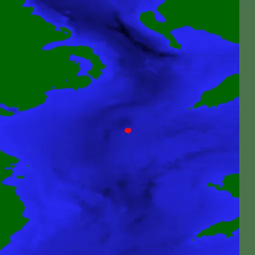
Image 1. A single source in the problem area.

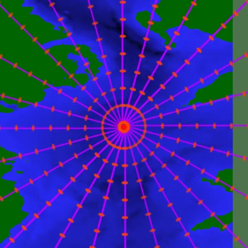
Image 2. Slices and solution points radiating from the source.

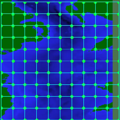
Image 3. The problem grid onto which levels are interpolated.

The overall sound levels are interpolated and summed over all active sources to produce the final grid.