Results

Overall Levels and Colour Scale

The Results Page gives control over the display of sound levels.

The current mapping of sound levels to colours is shown. Depending on whether Smooth result colours is selected under Preferences → Graphics, the results colours will either be displayed as solid colour bands or blend smoothly into one another.

To alter the limits or spacing between colour bands, click the Change limits button. This opens the level limits dialogue.

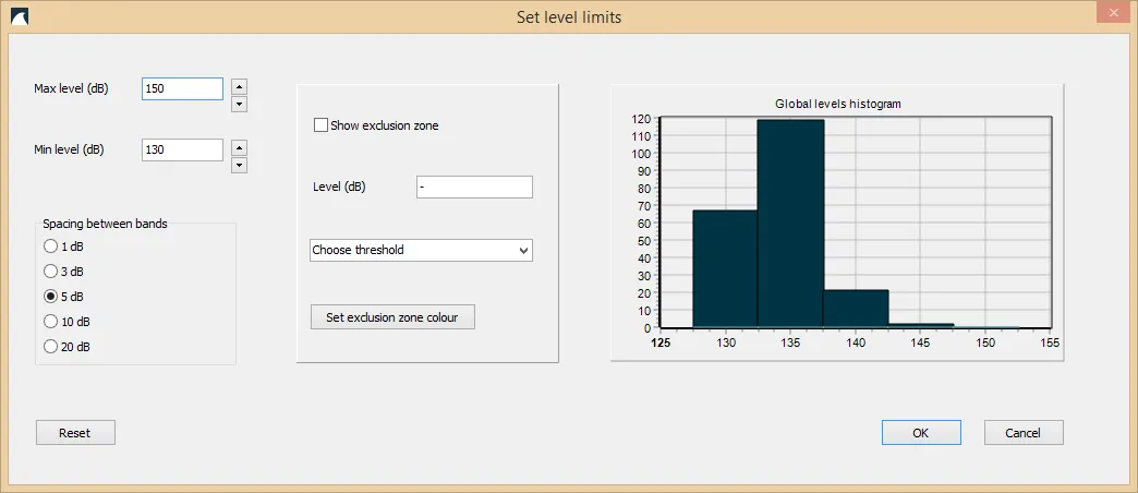Image 1: Set level limits window.

The maximum and minimum levels to display may be changed, and the spacing between adjacent bands can be set to 1, 3, 5, 10, or 20 dB.

Exclusion Zones

To display exclusion zones around sources, check the Show exclusion zone box. The exclusion level can be entered in the Level text box or selected from the dropdown menu, which contains thresholds from the database.

The main graphics area will show all areas where the currently selected minimum level is exceeded, coloured with the chosen colour. The colour may be changed with the Set exclusion zone colour button. If the Levels must decrease with distance from source option is not selected, this may cause problems for the exclusion zone drawing algorithm. Therefore, it is recommended that this option is selected when exclusion zones are desired.

If using predefined levels from the dropdown menu, please ensure that the variables in “Preferences” and “Sound levels display” are set to “Sound exposure level dB SELcum” and “Assessment period is set to 86400 seconds (24 hours) to comply with the assessment standards. Please also ensure that you understand the background of the weightings in [1]. Also, predefined impulsive thresholds are only available for time series sources, as they are not clearly defined in the above document. If you wish to assess a continuous sound source as impulsive, set the exclusion zone manually to the desired level as per [1].

To change the colours for the displayed results, click the Edit colours button. This shows the colour edit dialogue.

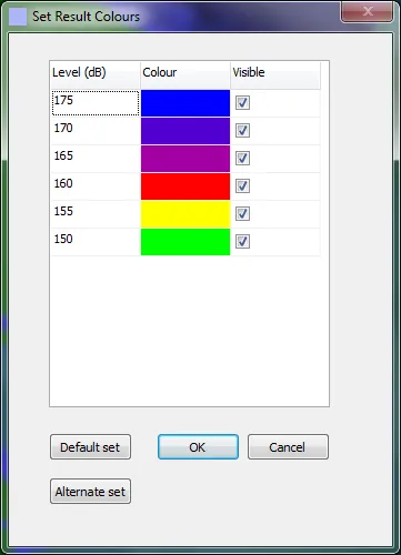Image 2: Colour edit dialogue window.

To change the colour for a particular band, click on that colour. To set a band to be not visible, uncheck the Visible box for that band.

Exporting Results

All export functions are accessed from the Export menu. The delimiter for text-based exports can be configured under Preferences → Exporting.

Image Export

The current scene can be exported as BMP, JPG, PNG, PDF, or GIF via Export current scene as. If the scene includes calculated sound levels, a colour scale bar is included. Text and logo overlays for exported images can be configured under Preferences → Exporting.

Sound Level Data

Menu item	Format	Content
Export max levels	Text (.txt)	Maximum level from all depths at each grid point
Export all levels	Text (.txt)	Levels at all grid points and all depth layers
Export all levels including spectra	Text (.txt)	As above, plus per-frequency-band levels
Export cross-section levels	Text (.txt)	Levels along the current cross-section
Export cross-section levels including spectra	Text (.txt)	As above, plus per-frequency-band levels
Copy visible levels as xy columns to clipboard	Clipboard	XYZ-format copy of currently visible levels

GIS Formats

ESRI ASCII grid (.asc):

Export currently visible levels in ESRI Ascii grid format — exports the current display layer as a single .asc file, geo-referenced to the project UTM zone
Export levels as ESRI Ascii grid file series — exports one .asc file per depth layer
Export bathymetry in ESRI Ascii grid format — exports the project bathymetry

XYZ (.xyz):

Export currently visible levels in xyz format — exports as comma-separated x, y, level columns with geographic coordinates

Shapefile (.shp):

Export contours as shapefile — exports sound level contours as vector LineStrings, with a .prj file for the project UTM zone

GeoJSON (.geojson):

Export contours as GeoJSON — exports contours as a GeoJSON FeatureCollection. Requires a valid UTM zone to be set

When exporting contours (shapefile or GeoJSON), only visible contour levels are included — hidden levels are excluded.

Exclusion Zone Export

The exclusion zone can be exported in three formats:

ESRI ASCII grid (.asc)
Shapefile (.shp, .shx, .dbf)
GeoJSON (.geojson) — requires valid UTM zone

Bathymetry Export

ESRI ASCII grid (.asc) — standard raster format
BTH format (.bth) — for compatibility with 3MB and ESME acoustic modelling tools. Requires a valid UTM zone, as the data is interpolated onto a lat/long grid

Weighted Levels Export

Export levels with weightings opens a dialog for batch-exporting levels across multiple species weighting curves. Select one or more weightings, choose an output format (text levels, max levels, ESRI grid, or shapefile contours), and set a filename prefix. A separate file is produced for each selected weighting.

Animated Results

The animated results tool creates a frame-by-frame animation showing how sound levels change as a moving source traverses its track. This is useful for visualising vessel passages, pile driving sequences, or any moving source scenario.

Access: Tools → Export → Animated results tool

Prerequisites:

The scenario must have been solved with results available
Exactly one moving source must be present in the scenario
Retain all calculated levels must be enabled for that source (see Sources)

If these conditions are not met, the Generate button will be disabled with an explanatory message.

Workflow:

Generate — click Generate to create animation frames. dBSea renders the sound level visualisation at each source position along the track, displaying a preview as it progresses. Generation can be cancelled at any time.
Set frame delay — enter the delay between frames in milliseconds (e.g. 100 ms = 10 frames per second).
Export — save as animated GIF or AVI video (Motion JPEG).

Reference

[1] Guidance for Assessing the Effects of Anthropogenic Sound on Marine Mammal Hearing, NOAA 2016